Tutorials & Examples

Example: Accessing the database and creating a figure

This example creates a figure comparing half-light radius and absolute magnitude of dwarf galaxies and star clusters. Note that as of v1.1.0 only the combined data files are located on the release pages (comb_all.csv).

Load required packages:

import numpy as np
import matplotlib.pyplot as plt
import astropy.table as table

Load the data from github:

## can be loaded from the release page (recommended method). Note that the release tag needs to be selected.
## this code block will load the latest version
version_number_string = table.Table.read('https://raw.githubusercontent.com/apace7/local_volume_database/main/code/release_version.txt', format='ascii.fast_no_header')['col1'][0]
print("verion", version_number_string)
## load combined table
comb_all = table.Table.read('https://github.com/apace7/local_volume_database/releases/download/'+version_number_string+'/comb_all.csv')

## select tables
dsph_mw = comb_all[comb_all['table'] == 'dwarf_mw']
dsph_m31 = comb_all[comb_all['table'] == 'dwarf_m31']
dsph_lf = comb_all[comb_all['table'] == 'dwarf_local_field']
gc_halo = comb_all[comb_all['table'] == 'gc_ambiguous']
gc_disk = comb_all[comb_all['table'] == 'gc_mw_new']
gc_harris = comb_all[comb_all['table'] == 'gc_harris']

Make a figure:

def const_mu(muV, rhalf):
    return muV - 36.57 - 2.5 * np.log10(2.*np.pi*rhalf**2)
x = np.arange(1, 1e4, 1)
for mu in [24, 26, 28, 30, 32]:
    plt.plot(x,  [const_mu(mu, i/1000.) for i in x], c='k', lw=2, ls=':')

plt.errorbar(dsph_mw['rhalf_sph_physical'], dsph_mw['M_V'], fmt='o', label=r'${\rm Dwarf~MW}$', )
plt.plot(dsph_m31['rhalf_sph_physical'], dsph_m31['M_V'], 'o', label=r'${\rm Dwarf~M31}$')
plt.plot(dsph_lf['rhalf_sph_physical'],dsph_lf['M_V'], 'o', label=r'${\rm Dwarf~LF}$')
plt.plot(gc_halo['rhalf_sph_physical'], gc_halo['M_V'], 'o',label=r'${\rm UFSC}$')
plt.plot(gc_disk['rhalf_sph_physical'], gc_disk['M_V'], 'o',label=r'${\rm GC~New}$')
plt.plot(gc_harris['rhalf_sph_physical'], gc_harris['M_V'], 'o',label=r'${\rm GC~Harris}$')
plt.gca().set_xscale('log')
plt.gca().invert_yaxis()
plt.gca().set_xlabel(r'$r_{1/2}~({\rm pc})$')
plt.gca().set_ylabel(r'$M_V$')
plt.legend(loc=(2))
plt.ylim(3, -20)
plt.xlim(1, 4e3)
plt.show()

Figure from the sample (this does include custom matplotlib stylefile and latex for the captions). I note that the name for one type of system in the catalog (labeled UFSC = ultra-faint star clusters) has been changed several times. In the majority of the documentation these are referred to as, new star cluster-like systems in Galactic halo and/or ambiguous systems (as in the nature of dwarf galaxy and star cluster is ambiguous).

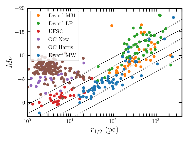
Example figure

Example Jupyter Notebooks

In addition to the example above, there are two folders with example ipython notebooks:

• general example notebooks

• LVDB overview plots

Some Recommendations

For scientific analysis, I would recommend a fixed tagged GitHub release of the LVDB.

## tagged GitHub release
version_number_string = table.Table.read('https://raw.githubusercontent.com/apace7/local_volume_database/main/code/release_version.txt', format='ascii.fast_no_header')['col1'][0]
print("verion", version_number_string)
## load combined table
comb_all = table.Table.read('https://github.com/apace7/local_volume_database/releases/download/'+version_number_string+'/comb_all.csv')

## or an older version
comb_all = table.Table.read('https://github.com/apace7/local_volume_database/releases/download/'+'v1.0.6'+'/comb_all.csv')

Interactive Website

An interactive version of the LVDB is available here: link (made by Katya Gozman).